Project: HiCAD 3-D
functions to derive splines from existing polylines. The spline will subsequently be located on the original c-edge.
Spline curves have the characteristic of running exactly through support points with minimum change of curvature, or meandering past them as smoothly as possible. The algorithms for the calculation of spline curves allow highly efficient interpolations.
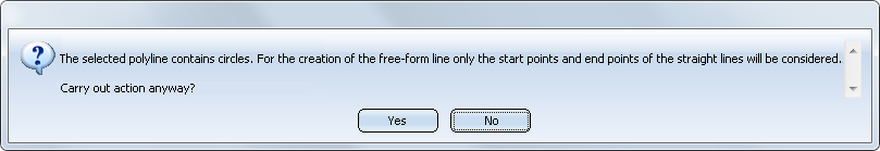
The functions listed above check whether the selected c-edge contains curves. If this is the case, an appropriate message will be issued, e.g.:
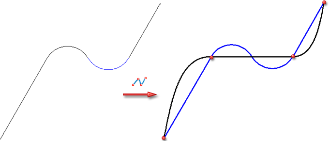
When you confirm this message with Yes, only the start points and end points of the straight line will be considered for the creation of the spline, as shown in the image below, where an Akima spline (including the arcs) has been derived from the sketch on the left hand side.
If you select No, the function will be cancelled, and no spline will be created.
To convert these polylines in such a way that splines can be directly derived from them, you can choose between the following options:
 function. Enter a suitable number of segments and activate the Convert curves into straight lines option.
  function to each curve of the polyline, activating the Replace with straight lines option.
  function.
Sketch > Draw > Freehand > Cubic spline 
The cubic spline is a third-degree polynomial which passes through the support points of the original composite edge. The individual segments/sections of the polynomial between the support points touch the support points "without bend". They are assigned a twice continuously differentiable smooth spline without explicit specification of tangential conditions. A cubic spline is interpolating!
If the polyline is closed, the continuous curve is automatically closed in the common start and end point with a smooth transition.
The Tangential cubic spline function is also used to create a cubic spline. However, the 1st derivation at the two edge points is equal to the direction between two consecutive points of the original polyline. This means that the directions of the first and last edge of the smoothed polyline are identical to the first and last edge of the original composite edge.
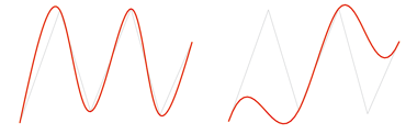
Left: Cubic spline; Right: Tangential cubic spline
Sketch > Draw > Freehand > Akima spline 
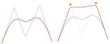
Unlike the cubic spline, the Akima spline is local. Although third-degree polynomials are also used, they are only once continuously differentiable in the total definition area. This means that the new composite edge is only defined by the support points in the immediate vicinity.
Moving a support point only affects the composite edge locally. In particular, a larger straight-line area is reproduced exactly via many support points in this area. By contrast, the cubic spline displays more wavy behaviour.
Sketch > Draw > Freehand > B-spline/NURBS 
A B-Spline is created via a sequence or a mesh of de Boor points, also called control points. The polyline through these points creates the de Boor polygon or control polygon. A B-spline is local, i.e. changes only have an effect in a certain parameter area. This enables any number of B-spline functions to be coupled to a B-spline curve. B-splines are not interpolating
NURB curves (Non Uniform Rational B-splines) are rational B-spline curves. They offer a wide range of options for the shaping of continuous curves. NURB curves can be assigned weights at the control points. They have a similar structure to B-spline curves. If the weight at the control points is 1, the rational B-spline curve changes to a normal B-spline. Conversely, every B-spline curve becomes a NURB curve if weights are assigned to its control points.
Left: B-spline, Right: The B-spline curve has been assigned weights at the highlighted points. The result is a NURB curve.

3-D Sketch (3-D) • Sketch Functions (3-D)
|
© Copyright 1994-2019, ISD Software und Systeme GmbH |